A special type of Artificial Neural Network

Background

Pioneered in 1982 by Finnish professor and researcher Dr. Teuvo Kohonen, a self-organising map is an unsupervised learning model, intended for applications in which maintaining a topology between input and output spaces is of importance. The notable characteristic of this algorithm is that the input vectors that are close — similar — in high dimensional space are also mapped to nearby nodes in the 2D space. It is in essence a method for dimensionality reduction, as it maps high-dimension inputs to a low (typically two) dimensional discretised representation and conserves the underlying structure of its input space.

A valuable detail is that the entire learning occurs without supervision i.e. the nodes are self-organising. They are also called feature maps, as they are essentially retraining the features of the input data, and simply grouping themselves according to the similarity between one another. This has a pragmatic value for visualising complex or large quantities of high dimensional data and representing the relationship between them into a low, typically two-dimensional, field to see if the given unlabelled data has any structure to it.

Structure

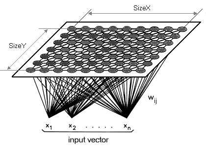
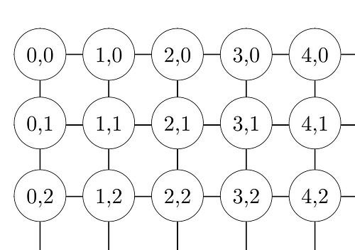
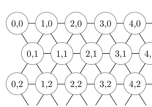
A Self-Organizing Map (SOM) differs from typical ANNs both in its architecture and algorithmic properties. Firstly, its structure comprises of a single-layer linear 2D grid of neurons, instead of a series of layers. All the nodes on this grid are connected directly to the input vector, but not to one another, meaning the nodes do not know the values of their neighbours, and only update the weight of their connections as a function of the given inputs. The grid itself is the map that organises itself at each iteration as a function of the input of the input data. As such, after clustering, each node has its own (i,j) coordinate, which allows one to calculate the Euclidean distance between 2 nodes by means of the Pythagorean theorem.

Properties

A Self-Organising Map, additionally, uses competitive learning as opposed to error-correction learning, to adjust it weights. This means that only a single node is activated at each iteration in which the features of an instance of the input vector are presented to the neural network, as all nodes compete for the right to respond to the input.

The chosen node — the Best Matching Unit (BMU) — is selected according to the similarity, between the current input values and all the nodes in the grid.

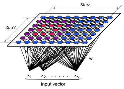
The node with the smallest Euclidean difference between the input vector and all nodes is chosen, along with its neighbouring nodes within a certain radius, to have their position slightly adjusted to match the input vector.

By going through all the nodes present on the grid, the entire grid eventually matches the complete input dataset, with similar nodes grouped together towards one area, and dissimilar ones separated.

Variables

• t is the current iteration
• n is the iteration limit, i.e. the total number of iterations the network can undergo
• λ is the time constant, used to decay the radius and learning rate
• i is the row coordinate of the nodes grid
• j is the column coordinate of the nodes grid
• d is the distance between a node and the BMU
• w is the weight vector
• w_ij(t) is the weight of the connection between the nodes i,j in the grid, and the input vector’s instance at the iteration t
• x is the input vector
• x(t) is the input vector’s instance at iteration t
• α(t) is the learning rate, decreasing with time in the interval [0,1], to ensure the network converges.
• β_ij(t) is the neighbourhood function, monotonically decreasing and representing a node i, j’s distance from the BMU, and the influence it has on the learning at step t.
• σ(t) is the radius of the neighbourhood function, which determines how far neighbour nodes are examined in the 2D grid when updating vectors. It is gradually reduced over time.

Algorithm

1. Initialise each node’s weight w_ij to a random value
2. Select a random input vector x_k
3. Repeat point 4. and 5. for all nodes in the map:
4. Compute Euclidean distance between the input vector x(t) and the weight vector w_ij associated with the first node, where t, i, j = 0.
5. Track the node that produces the smallest distance t.
6. Find the overall Best Matching Unit (BMU), i.e. the node with the smallest distance from all calculated ones.
7. Determine topological neighbourhood βij(t) its radius σ(t) of BMU in the Kohonen Map
8. Repeat for all nodes in the BMU neighbourhood: Update the weight vector w_ij of the first node in the neighbourhood of the BMU by adding a fraction of the difference between the input vector x(t) and the weight w(t) of the neuron.
9. Repeat this whole iteration until reaching the chosen iteration limit t=n

Step 1 is the initialisation phase, while step 2–9 represent the training phase.

Formulas

The updates and changes to the variables are done according to the following formulas:

The weights within the neighbourhood are updated as:

The first equation tells us that the new updated weight w_ij (t + 1) for the node i, j is equal to the sum of old weight w_ij(t) and a fraction of the difference between the old weight and the input vector x(t). In other words, the weight vector is ‘moved’ closer towards the input vector. Another important element to note is that the updated weight will be proportional to the 2D distance between the nodes in the neighbourhood radius and the BMU.

Furthermore, the same equation 3.1 does not account for the influence of the learning being proportional to the distance a node is from the BMU. The updated weight should take into factor that the effect of the learning is close to none at the extremities of the neighbourhood, as the amount of learning should decrease with distance. Therefore, the second equation adds the extra neighbourhood function factor of βij(t), and is the more precise in-depth one.

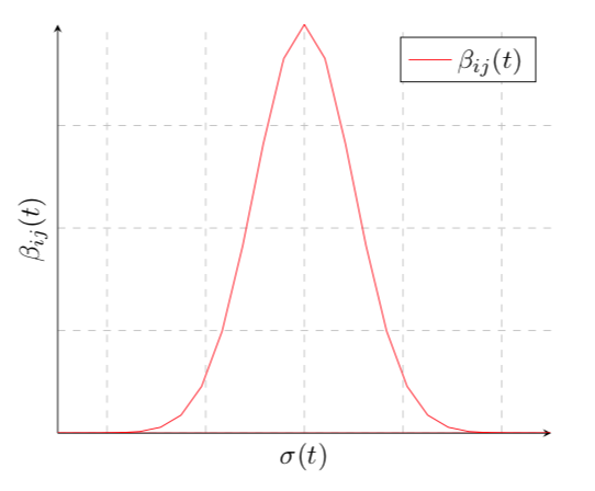
The radius and learning rate are both similarly and exponentially decayed with time.

The neighbourhood function’s influence β_i(t) is calculated by:

The Euclidean distance between each node’s weight vector and the current input instance is calculated by the Pythagorean formula.

The BMU is selected from all the node’s calculated distances as the one with the smallest.

Further Reading

• A deeper reading on all aspects of the algorithm: https://eklavyafcb.github.io/som.html
• A good implementation on the algorithm can be found at: https://github.com/EklavyaFCB/EMNIST-Kohonen-SOM